20250202 모각코 활동 4회차
오늘의 목표 : Pandas 공부와 타이타닉 데이터 분석
Pandas 🐼
판다스 특징
- 판다스(Pandas) : 파이썬에서의 데이터 분석과 처리를 위해 사용되는 라이브러리.
- 엑셀, CSV, SQL 같은 다양한 형식의 데이터를 쉽게 다룰 수 있음.
- numpy기반으로 만들어져 빠르고 효율적임.
주요 데이터 구조와 불러오기
Series (1차원 데이터)
- 리스트나 배열과 비슷하지만, 인덱스를 가질 수 있음.
data = pd.Series([10, 20, 30, 40], index=['A', 'B', 'C', 'D'])
DataFrame (2차원 데이터)
- 표 형태의 데이터 구조로, 행과 열로 구성됨.
data = {'Name': ['Alice', 'Bob', 'Charlie'], 'Age': [25, 30, 35], 'Score': [85, 90, 95]}
데이터 불러오기
.read_csv('파일경로.csv')  # CSV 파일 불러오기
.read_excel('파일경로.xlsx') # 엑셀 파일 불러오기
주요 함수
.info()  # 데이터 요약 정보
.describe()  # 수치형 데이터 통계 요약 (이 때, include = 'object' 라는 파라미터를 넣어주면, 범주형 변수에 대한 통계정보를 볼 수 있음. )
.shape  # (행, 열) 크기 확인
.columns  # 컬럼(열) 이름 확인
.dtypes  # 데이터 타입 확인
.isnull().sum()  # 결측치(NaN) 개수 확인
.head()  # 상위 5개 행 출력
.tail()  # 하위 5개 행 출력
.dropna()  # 결측치가 하나라도 있는 행 삭제
.
.
.
등등...
타이타닉 데이터 분석
데이터 준비
# 필요한 모듈 불러오기
import pandas as pd
import matplotlib.pyplot as plt
import seaborn as sns

# 데이터 불러오기
df = sns.load_dataset('titanic')

# 데이터 기본 정보 확인
print(df.info())
print(df.isnull().sum())  # 결측치 확인

# 결측치 처리 (결측치가 하나라도 있는 행은 그냥 없애버릴것이다~!)
df = df.dropna()
df = df.reset_index(drop=True)  # 인덱스 정리
결과
<class 'pandas.core.frame.DataFrame'>
RangeIndex: 891 entries, 0 to 890
Data columns (total 15 columns):
 #   Column       Non-Null Count  Dtype
---  ------       --------------  -----
 0   survived     891 non-null    int64
 1   pclass       891 non-null    int64
 2   sex          891 non-null    object
 3   age          714 non-null    float64
 4   sibsp        891 non-null    int64
 5   parch        891 non-null    int64
 6   fare         891 non-null    float64
 7   embarked     889 non-null    object
 8   class        891 non-null    category
 9   who          891 non-null    object
 10  adult_male   891 non-null    bool
 11  deck         203 non-null    category
 12  embark_town  889 non-null    object
 13  alive        891 non-null    object
 14  alone        891 non-null    bool
dtypes: bool(2), category(2), float64(2), int64(4), object(5)
memory usage: 80.7+ KB
None
survived         0
pclass           0
sex              0
age            177
sibsp            0
parch            0
fare             0
embarked         2
class            0
who              0
adult_male       0
deck           688
embark_town      2
alive            0
alone            0
dtype: int64
기본 통계 분석
print(df.describe())
print(df.describe(include = 'object'))  # 범주형 변수에 대한 통계정보
결과
         survived      pclass         age       sibsp       parch        fare
count  182.000000  182.000000  182.000000  182.000000  182.000000  182.000000
mean     0.675824    1.192308   35.623187    0.467033    0.478022   78.919735
std      0.469357    0.516411   15.671615    0.645007    0.755869   76.490774
min      0.000000    1.000000    0.920000    0.000000    0.000000    0.000000
25%      0.000000    1.000000   24.000000    0.000000    0.000000   29.700000
50%      1.000000    1.000000   36.000000    0.000000    0.000000   57.000000
75%      1.000000    1.000000   47.750000    1.000000    1.000000   90.000000
max      1.000000    3.000000   80.000000    3.000000    4.000000  512.329200
         sex embarked  who  embark_town alive
count    182      182  182          182   182
unique     2        3    3            3     2
top     male        S  man  Southampton   yes
freq      94      115   87          115   123
생존률 분석
# 성별에 따른 생존률
print(df.groupby('sex')['survived'].mean() * 100)

# 객실 등급에 따른 생존률
print(df.groupby('pclass')['survived'].mean() * 100)

# 연령대별 생존률
print(df.groupby('age')['survived'].mean() * 100)
결과
sex
female    93.181818
male      43.617021
Name: survived, dtype: float64

pclass
1    67.515924
2    80.000000
3    50.000000
Name: survived, dtype: float64

age
0.92     100.000000
1.00     100.000000
2.00      33.333333
3.00     100.000000
4.00     100.000000
            ...
64.00      0.000000
65.00      0.000000
70.00      0.000000
71.00      0.000000
80.00    100.000000
Name: survived, Length: 63, dtype: float64
상관관계 분석과 시각화
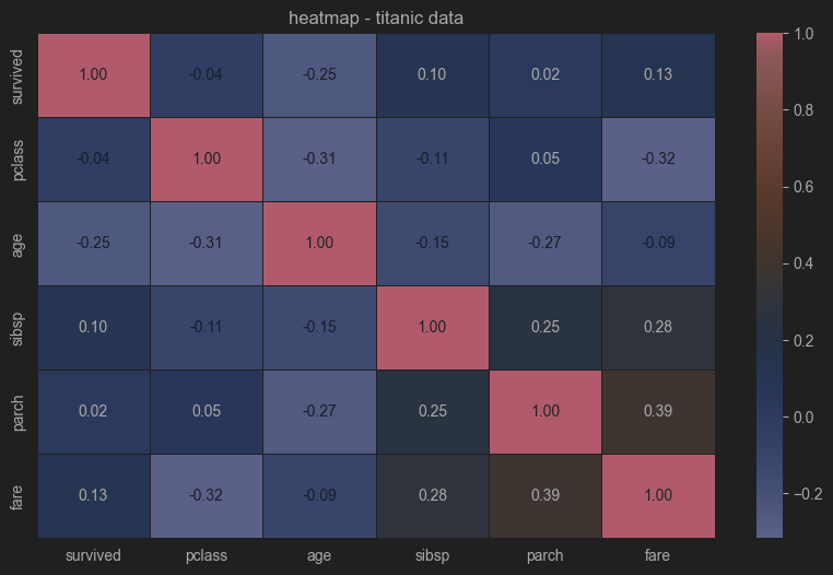
corr_data = df.select_dtypes(include=['number']).corr()  # 숫자형 데이터만 추출하여 상관관계 분석

# 상관관계 시각화
plt.figure(figsize=(10, 6))
sns.heatmap(corr_data, annot=True, cmap='coolwarm', fmt=".2f", linewidths=0.5)
plt.title("heatmap - titanic data")
plt.show()
# 주요 변수들간의 상관관계 시각화
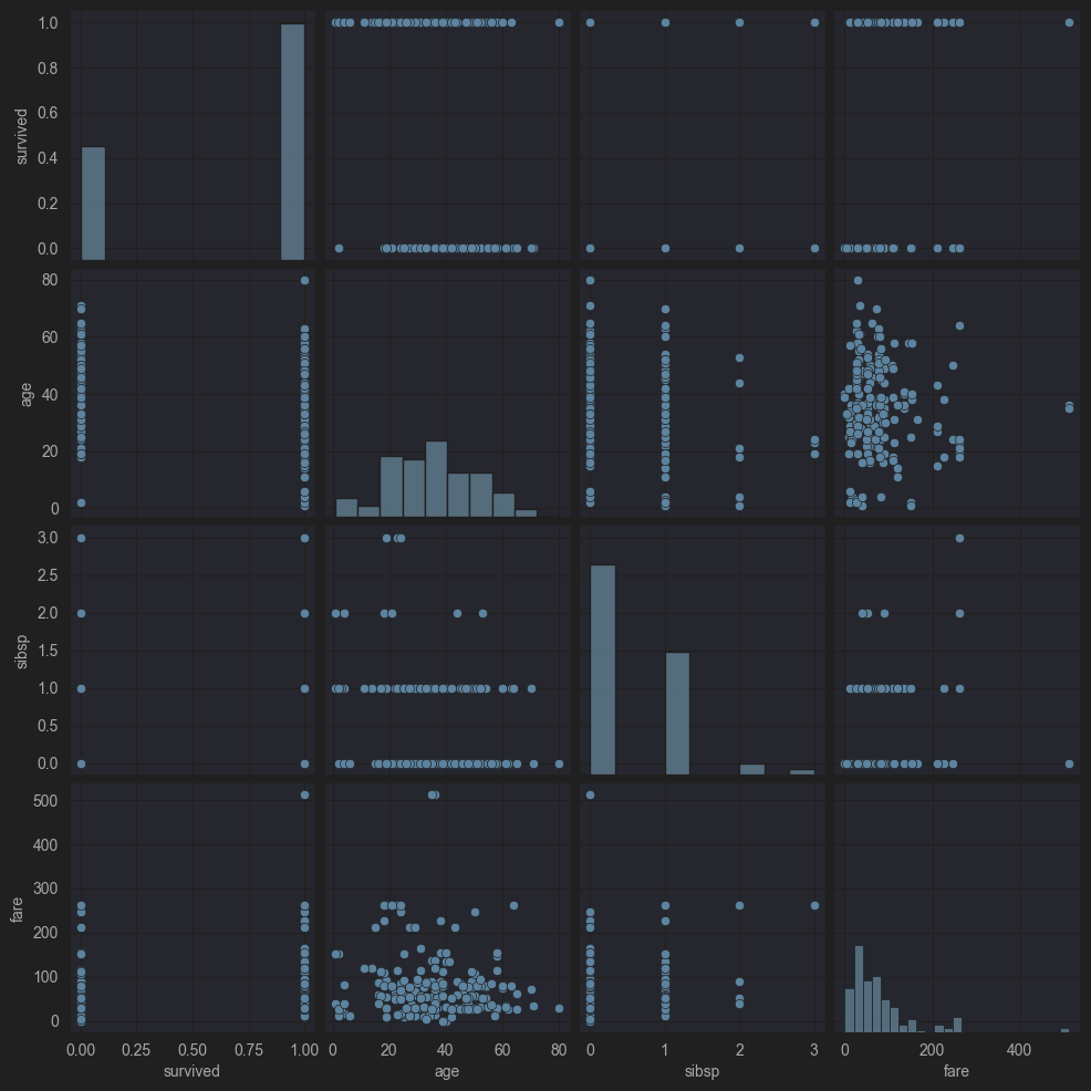
sns.pairplot(df[['survived', 'age', 'sibsp', 'fare']])
plt.show()